BIA CAE2 Question Bank with Answers
Questions
- BIA CAE2 Question Bank with Answers
- Questions
- Answers
- 1. State regression. List and explain types of regression - Ans1
- 2. With suitable examples, elaborate on the following terms: SST (Sum of Squares Total), SSR (Sum of Squares Regression), SSE (Sum of Squares Error) - Ans2
- 3. Discuss the Significance of P-Value in statistics - Ans3
- 4. Explain the applications of Multiple Linear Regression - Ans4
- 5. Differentiate between clustering and classification - Ans5
- 6. Explain K-means clustering with a suitable diagram - Ans6
- 7. Explain types of clustering in analytics - Ans7
- 8. List and explain the Pros and Cons of K-Means Clustering - Ans8
- 9. Distinguish between Clustering and Regression - Ans9
- 10. Explain Market Segmentation with Cluster Analysis - Ans10
- 11. Explain types of Classification (any 2) - Ans11
- 12. Elaborate with suitable example Classification Applications - Ans12
- 13. Explain sigmoid curve in Logistic Regression - Ans13
- 14. Explain Classification using SVM - Ans14
- 15. Explain K-nearest neighbor application in detail - Ans15
- 16. How Decision Tree algorithm works - Ans16
- 17. Explain R-Square
- 18. Discuss Adjusted R-Squared with a suitable example - Ans18
Answers
1. State regression. List and explain types of regression
Ans1
Regression is a statistical method used to model the relationship between a dependent variable and one or more independent variables. It is often used for predicting or explaining the variation in the dependent variable based on the values of the independent variables. There are several types of regression models:
-
Linear Regression: Linear regression aims to establish a linear relationship between the dependent variable and one or more independent variables. It's used when the relationship between variables is approximately linear.
-
Multiple Linear Regression: This extends linear regression to multiple independent variables. It's suitable when the dependent variable is influenced by more than one predictor.
-
Polynomial Regression: Polynomial regression is used when the relationship between the dependent variable and the independent variable(s) can be better represented by a polynomial equation (e.g., quadratic or cubic).
-
Logistic Regression: Unlike linear regression, logistic regression is used when the dependent variable is binary (e.g., 0 or 1). It models the probability of an event occurring.
-
Ridge Regression and Lasso Regression: These are variations of linear regression that include regularization terms to prevent overfitting by adding penalty to the model coefficients.
-
Decision Tree Regression: Decision tree regression involves constructing a decision tree to predict the dependent variable. It's non-linear and can capture complex relationships.
-
Support Vector Regression (SVR): SVR is used for regression tasks and aims to find a hyperplane that best fits the data while minimizing the error.
-
Time Series Regression: This type is used when the data is collected over time, and the goal is to predict future values based on past observations.
2. With suitable examples, elaborate on the following terms: SST (Sum of Squares Total), SSR (Sum of Squares Regression), SSE (Sum of Squares Error)
Ans2
SST (Sum of Squares Total): SST is a measure of the total variation in the dependent variable. It quantifies how much the data points deviate from the mean of the dependent variable. It can be calculated as the sum of the squares of the differences between each data point and the mean of the dependent variable.
- Example: In a study of student test scores, SST would quantify the total variation in test scores across all students, regardless of any predictors (independent variables).
SSR (Sum of Squares Regression): SSR measures the variation in the dependent variable that is explained by the regression model. It quantifies how well the independent variables account for the changes in the dependent variable. SSR is calculated as the sum of the squares of the differences between the predicted values (obtained from the regression model) and the mean of the dependent variable.
- Example: In a multiple linear regression model, SSR would quantify how much of the variation in student test scores can be attributed to predictors like study hours, attendance, and previous test scores.
SSE (Sum of Squares Error): SSE represents the unexplained variation or the residual variation in the dependent variable. It measures the difference between the actual values of the dependent variable and the predicted values from the regression model.
- Example: In the same multiple linear regression model, SSE would represent the variation in student test scores that cannot be explained by study hours, attendance, and previous test scores. It includes random or unmodeled factors affecting test scores.
3. Discuss the Significance of P-Value in statistics
Ans3
The p-value (probability value) is a critical concept in statistics, particularly in hypothesis testing. It quantifies the evidence against a null hypothesis. Here's its significance:
-
Hypothesis Testing: In hypothesis testing, the p-value helps determine whether the observed data provides enough evidence to reject the null hypothesis. The null hypothesis typically represents a default assumption of no effect or no difference.
-
Interpretation: A low p-value (typically less than a significance level, such as 0.05) suggests that the observed data is unlikely under the null hypothesis. This leads to the rejection of the null hypothesis in favor of an alternative hypothesis, indicating that there may be a significant effect or relationship.
-
Confidence in Results: A low p-value indicates that the results are statistically significant, which means that the observed effect is unlikely to have occurred by random chance alone. This provides confidence in the validity of the findings.
-
Adjusting for Type I Error: Researchers choose a significance level (alpha) to control the risk of making a Type I error (incorrectly rejecting a true null hypothesis). The p-value allows them to assess whether the observed data meets this predetermined threshold.
-
Caution: However, it's important to note that a low p-value does not prove the practical or clinical significance of an effect. It only indicates that the effect is statistically significant. Researchers should also consider effect size and context.
4. Explain the applications of Multiple Linear Regression
Ans4
Multiple Linear Regression is a versatile statistical method with various applications, including:
-
Economics: Predicting factors affecting economic indicators like GDP, inflation, or unemployment by considering multiple variables such as interest rates, government spending, and consumer confidence.
-
Marketing: Estimating the impact of various marketing strategies (e.g., advertising spend, pricing, and product features) on sales or customer satisfaction.
-
Medicine and Healthcare: Predicting patient outcomes based on multiple factors, like age, weight, blood pressure, and medical history. It's also used for disease prevalence studies.
-
Finance: Modeling stock prices or portfolio performance using factors like interest rates, company performance metrics, and market indices.
-
Environmental Science: Assessing the relationship between environmental variables (e.g., temperature, humidity, and pollution levels) and their impact on natural phenomena, such as plant growth or climate change.
-
Social Sciences: Analyzing the impact of various sociological factors on social phenomena, like crime rates, education outcomes, or population growth.
-
Engineering: Predicting the behavior of complex systems or products based on multiple design variables, material properties, and operating conditions.
-
Manufacturing and Quality Control: Identifying factors influencing product quality and optimizing production processes.
-
Education: Analyzing student performance using multiple variables like teacher experience, class size, and resource allocation.
-
Real Estate: Estimating property prices based on attributes like location, size, number of bedrooms, and other features.
5. Differentiate between clustering and classification
Ans5
Clustering:
- Purpose: Clustering is an unsupervised learning technique used to group similar data points based on their intrinsic characteristics.
- Training Data: Clustering does not require labeled data or predefined categories.
- Output: The output of clustering is the grouping of data points into clusters, which may not have clear, predefined names or labels.
- Example: Grouping customers based on their purchasing behavior without knowing in advance which groups exist.
Classification:
- Purpose: Classification is a supervised learning technique used to assign predefined labels or categories to data points based on their features.
- Training Data: Classification requires labeled training data with examples of each class to learn from.
- Output: The output of classification is a prediction or assignment of a specific category or label to each data point.
- Example: Assigning an email as "spam" or "not
6. Explain K-means clustering with a suitable diagram
Ans6
K-means clustering is a type of unsupervised machine learning algorithm used to group data points into clusters based on their similarities. The algorithm aims to partition data into clusters in such a way that each data point belongs to the cluster with the nearest mean. Here's how it works:
- Step 1: Initialize the process by selecting the number of clusters (K) you want to create.
-
Step 2: Randomly select K data points as the initial centroids (representative points) for each cluster.
-
Step 3: Assign each data point to the nearest centroid, forming K clusters.
-
Step 4: Recalculate the centroid of each cluster by taking the mean of all data points within the cluster.
-
Step 5: Repeat steps 3 and 4 until the centroids no longer change significantly, or a predefined number of iterations is reached.
Here's a suitable diagram to visualize K-means clustering:
K-means clustering diagram
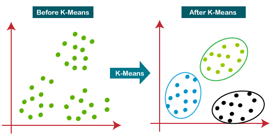
In the diagram, you can see how data points are initially assigned to clusters based on their proximity to the centroids. The centroids are recalculated, and the assignment process is repeated until convergence is achieved.
7. Explain types of clustering in analytics
Ans7
There are several types of clustering algorithms in analytics:
-
K-means clustering: As explained above, it partitions data into K clusters based on similarity.
-
Hierarchical clustering: It creates a hierarchy of clusters, starting with individual data points and combining them into larger clusters.
-
DBSCAN (Density-Based Spatial Clustering of Applications with Noise): It clusters data based on density, making it suitable for data with irregular shapes and varying densities.
-
Agglomerative clustering: A type of hierarchical clustering, it starts with each data point as a single cluster and successively merges them into larger clusters.
-
Spectral clustering: This method uses eigenvalues of similarity matrices to perform clustering, often used for image segmentation and text document clustering.
-
Fuzzy clustering: Unlike K-means, where data points belong to a single cluster, fuzzy clustering allows data points to belong to multiple clusters with varying degrees of membership.
-
Model-based clustering: It assumes that data is generated by a mixture of probability distributions and attempts to find the best-fit model for the data.
8. List and explain the Pros and Cons of K-Means Clustering
Ans8
Pros:
- Simplicity: K-means is easy to understand and implement.
- Speed: It is computationally efficient, making it suitable for large datasets.
- Scalability: It can handle high-dimensional data.
- Versatility: Works well with various types of data, such as numeric, categorical, or mixed.
Cons:
- Sensitive to Initial Centroids: The final clustering can vary depending on the initial placement of centroids.
- Requires Predefined K: The number of clusters, K, needs to be known or determined beforehand.
- Assumes Spherical Clusters: K-means may not perform well when clusters are non-spherical or have different sizes.
- May Converge to Local Optima: The algorithm may get stuck in suboptimal cluster assignments.
- Outliers Impact Results: Outliers can significantly affect the cluster centroids and, thus, the clustering.
9. Distinguish between Clustering and Regression
Ans9
| Feature | Clustering | Regression |
|---|---|---|
| Objective | Group similar data points together based on their characteristics or features. | Model the relationship between input variables and a target variable, making predictions or estimating the target variable. |
| Output | Produces clusters or groups of data points without any prediction or estimation of a target variable. | Produces a predictive model that can be used to make continuous numerical predictions. |
| Supervision | Unsupervised learning - no labeled target variable is used during the process. | Supervised learning - relies on labeled data with a known target variable. |
| Use Case | Used for pattern recognition, data exploration, and finding inherent structure in data. | Used for prediction, forecasting, and understanding the relationships between variables. |
| Examples | Customer segmentation, image segmentation, anomaly detection. | Predicting house prices based on features like square footage and location, forecasting sales based on historical data, estimating a person's age based on demographic information. |
10. Explain Market Segmentation with Cluster Analysis
Ans10
Market segmentation is a crucial marketing strategy that involves dividing a market into distinct groups or segments, each with specific characteristics and needs. Cluster analysis is a valuable tool for market segmentation. Here's how it works:
-
Data Collection: Gather relevant data about customers, such as demographics, behavior, preferences, or purchase history.
-
Data Preprocessing: Clean and prepare the data, ensuring it's ready for analysis.
-
Feature Selection: Choose the most relevant features for segmentation.
-
Cluster Analysis: Use a clustering algorithm (like K-means) to group customers with similar characteristics into segments.
-
Segment Profiling: Analyze the characteristics of each segment to understand their unique attributes, such as age, income, preferences, and behaviors.
-
Segment Targeting: Tailor marketing strategies and products/services to cater to the specific needs and preferences of each segment.
Evaluation: Continuously monitor and evaluate the effectiveness of the segmentation and marketing efforts.
Market segmentation with cluster analysis allows businesses to better target their marketing efforts, create personalized campaigns, and increase customer satisfaction by providing relevant products and services. It helps in optimizing resource allocation and improving the overall marketing strategy.
11. Explain types of Classification (any 2)
Ans11
Classification is a supervised machine learning task where the goal is to categorize data points into predefined classes or categories. Here are two common types of classification:
a. Binary Classification: Binary classification is the simplest form of classification where data is divided into two classes or categories. The goal is to determine which of the two categories a given data point belongs to. A classic example of binary classification is email spam detection, where emails are categorized as either spam or not spam (ham).
Example: In a medical diagnosis scenario, you can use binary classification to determine whether a patient has a specific disease (e.g., diabetes) or not.
b. Multiclass Classification: In multiclass classification, the data is divided into more than two classes, and the goal is to assign each data point to one of the multiple classes. It's commonly used in scenarios where there are more than two possible outcomes.
Example: Image classification, where you classify images of animals into categories like "cat," "dog," "elephant," and so on.
12. Elaborate with suitable example Classification Applications
Ans12
Classification has a wide range of real-world applications. Here are two examples:
a. Sentiment Analysis: Sentiment analysis, also known as opinion mining, is a classification task that involves determining the sentiment or emotion expressed in a piece of text, such as a tweet, product review, or news article. The classes can be positive, negative, or neutral sentiments.
Example: Analyzing customer reviews of a product to classify them as positive, negative, or neutral. This can help companies understand customer opinions and make improvements to their products.
b. Fraud Detection: In the finance industry, classification is used for fraud detection. Given a transaction, the goal is to classify it as either legitimate or fraudulent. The classes are typically "fraud" or "non-fraud."
Example: Banks and credit card companies use classification models to detect unusual patterns or anomalies in financial transactions and flag potential fraudulent activities for further investigation.
13. Explain sigmoid curve in Logistic Regression
Ans13
In logistic regression, the sigmoid curve, also known as the logistic function, is used to model the relationship between the dependent variable (usually binary, like 0 or 1) and one or more independent variables. The sigmoid function is an S-shaped curve that maps any real-valued number to a value between 0 and 1.
The formula for the sigmoid function is:
P(Y=1∣X)=11+e−zP(Y=1∣X)=1+e−z1
Here:
- P(Y=1∣X)P(Y=1∣X) represents the probability of the dependent variable (Y) being 1 given the input features (X).
- zz is a linear combination of the input features, z=β0+β1X1+β2X2+…+βnXnz=β0+β1X1+β2X2+…+βnXn.
- ee is the base of the natural logarithm.
The sigmoid curve looks like an S-shape, and it has the property that it asymptotically approaches 0 as zz goes to negative infinity and approaches 1 as zz goes to positive infinity. This makes it suitable for modeling probabilities in binary classification problems.
14. Explain Classification using SVM
Ans14
Support Vector Machine (SVM) is a powerful classification algorithm that works by finding a hyperplane that best separates data points into different classes while maximizing the margin between the classes. Here's how classification using SVM works:
-
Data Preparation: You start with a labeled dataset where each data point belongs to one of two classes (binary classification) or multiple classes (multiclass classification).
-
Feature Selection/Extraction: Choose relevant features from the data or perform feature engineering if needed.
-
Choosing the Kernel: SVM uses a kernel function to map the data into a higher-dimensional space, where a hyperplane can be found to separate the classes. Common kernel functions include linear, polynomial, and radial basis function (RBF).
-
Training the Model: SVM finds the optimal hyperplane that maximizes the margin between classes. Support vectors, which are data points closest to the decision boundary, play a critical role in this process.
-
Testing/Predicting: Once the SVM model is trained, you can use it to classify new, unseen data points by mapping them into the same feature space and determining which side of the hyperplane they fall on.
SVMs are effective for handling high-dimensional data and can handle both linearly separable and non-linearly separable datasets by using appropriate kernels. They are commonly used in image classification, text classification, and bioinformatics, among other applications.
15. Explain K-nearest neighbor application in detail
Ans15
K-Nearest Neighbors (K-NN) is a simple yet effective classification algorithm based on the principle that data points in the same class tend to be close to each other in the feature space. Here's how K-NN works and an application example:
Working of K-NN:
-
Training: The K-NN algorithm begins with a training dataset, where each data point is associated with a class label.
-
Distance Metric: You need to choose a distance metric, often Euclidean distance, to measure the similarity or dissimilarity between data points.
-
Prediction: When you want to classify a new data point, K-NN looks at the K nearest data points in the training dataset, where K is a user-defined parameter. The majority class among the K-nearest neighbors is assigned as the predicted class for the new data point.
K-NN Application Example: Imagine you have a dataset of customer information, including age and income, and you want to classify customers into two categories: "high-value" and "low-value" customers. You can use K-NN for this task.
-
Training: You use the training data, where each customer is labeled as "high-value" or "low-value" based on historical data.
-
Distance Metric: You choose a distance metric (e.g., Euclidean distance) to measure the similarity between customers based on their age and income.
-
Prediction: When a new customer enters the store and provides their age and income, K-NN calculates the distances to the K-nearest customers in the training dataset. If, for instance, the majority of the K-nearest neighbors are labeled as "high-value," the new customer is classified as a "high-value" customer.
K-NN is used in various applications, including recommendation systems, image classification, and anomaly detection, where data points with similar characteristics are expected to belong to the same class or category.
16. How Decision Tree algorithm works
Ans16
Decision Trees are a popular machine learning algorithm used for both classification and regression tasks. They work by recursively splitting the dataset into subsets based on the most significant attribute at each node, ultimately creating a tree-like structure. Here's a detailed explanation of how the Decision Tree algorithm works:
-
Step 1: Data Preparation: Initially, you start with a dataset containing various features and a target variable. The algorithm requires labeled data, meaning each data point has a known outcome that the model tries to predict.
-
Step 2: Root Node Selection: The Decision Tree begins with the root node, representing the entire dataset. It evaluates all available features and selects the one that best splits the data into subsets based on some criteria. The criteria can vary, but commonly used ones include Gini impurity, entropy, or mean squared error, depending on whether you're doing classification or regression.
-
Step 3: Splitting: Once the feature for the root node is selected, the dataset is divided into subsets based on the feature's values. For categorical data, it creates branches for each category; for continuous data, it selects a threshold value. These splits continue recursively for each branch, creating child nodes.
-
Step 4: Recursive Splitting: The algorithm continues splitting the data at each node based on the feature that minimizes the chosen impurity criterion. This process is repeated until a stopping condition is met. Common stopping conditions include reaching a predetermined depth, a minimum number of samples in a node, or when further splits do not improve the model's performance significantly.
-
Step 5: Leaf Node Assignment: As the tree grows, it creates leaf nodes representing the final predictions. For classification tasks, the majority class in a leaf node is the predicted class, while for regression, it's the average of the target values in that node.
-
Step 6: Prediction: To make predictions, you follow the path from the root to a leaf node based on the feature values of the input data. The value in the leaf node is then returned as the model's prediction.
-
Step 7: Pruning (Optional): To prevent overfitting, Decision Trees can be pruned by removing branches that do not significantly improve model performance. Pruning helps create a more generalized and interpretable tree.
Decision Trees are interpretable and easy to visualize, making them valuable for understanding the decision-making process within the model. However, they can be prone to overfitting, which can be mitigated with techniques like pruning or using ensemble methods like Random Forests.
17. Explain R-Square
R-squared, also known as the coefficient of determination, is a statistical measure used to assess the goodness-of-fit of a regression model. It quantifies the proportion of the variance in the dependent variable (the target) that is explained by the independent variables (features) in the model. R-squared values range from 0 to 1, where:
- R-squared = 0: The model does not explain any variance in the target variable.
- R-squared = 1: The model perfectly explains the variance in the target variable.
Mathematically, R-squared is defined as:
R2=1−SSRSSTR2=1−SSTSSR
-
SSR (Sum of Squared Residuals): This represents the sum of the squared differences between the observed values and the values predicted by the regression model. It quantifies the unexplained variance.
-
SST (Total Sum of Squares): This represents the sum of the squared differences between the observed values and the mean of the observed values. It quantifies the total variance in the target variable.
R-squared tells you how well the independent variables in your model explain the variation in the dependent variable. A higher R-squared value indicates a better fit, but a very high R-squared doesn't necessarily mean a good model if it's overfitting. It's essential to consider other evaluation metrics and the context of your problem when interpreting R-squared.
18. Discuss Adjusted R-Squared with a suitable example
Ans18
Adjusted R-squared is a modified version of the regular R-squared that adjusts for the number of predictors in a regression model. It is particularly useful when dealing with multiple regression models where more than one independent variable is considered. Adjusted R-squared penalizes the inclusion of irrelevant predictors, preventing the inflation of R-squared due to the addition of variables that do not contribute significantly to the model's performance.
The formula for Adjusted R-squared is:
AdjustedR2=1−(1−R2)⋅(n−1)n−k−1AdjustedR2=1−n−k−1(1−R2)⋅(n−1)
Where:
- R2R2 is the regular R-squared.
- nn is the number of data points.
- kk is the number of predictors (independent variables).
Let's illustrate Adjusted R-squared with an example:
Suppose you are building a multiple linear regression model to predict a person's income based on three features: education level, years of experience, and age. You have collected data from 100 individuals. The regular R-squared of your model is 0.75.
R-squared = 0.75
In this case, R-squared indicates that 75% of the variance in income is explained by these three predictors.
Now, to calculate the Adjusted R-squared, you consider the number of predictors (k = 3) and the number of data points (n = 100). Plugging these values into the formula:
AdjustedR2=1−(1−0.75)⋅(100−1)100−3−1=0.7237AdjustedR2=1−100−3−1(1−0.75)⋅(100−1)=0.7237
So, the Adjusted R-squared is 0.7237. This adjusted value takes into account the number of predictors and provides a more accurate measure of how well the model fits the data, accounting for potential overfitting. In this example, an Adjusted R-squared of 0.7237 means that 72.37% of the variance in income is explained by the model while considering the number of predictors.