Unit 3: Relational Database Design

Functional Dependency (FD) Basic concepts

Functional dependency (FD) is a set of constraints between two attributes in a relation. Functional dependency says that if two tuples have same values for attributes A1, A2,..., An, then those two tuples must have to have same values for attributes B1, B2, ..., Bn.

The functional dependency is a relationship that exists between two attributes. It typically exists between the primary key and non-key attribute within a table.

For Example Assume we have an employee table with attributes: Emp_Id, Emp_Name, Emp_Address.

Here Emp_Id attribute can uniquely identify the Emp_Name attribute of employee table because if we know the Emp_Id, we can tell that employee name associated with it.

Functional dependency can be written as:

Emp_Id → Emp_Name

Types of Functional Dependencies

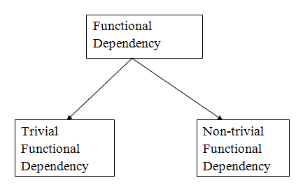
1.Trivial functional dependency

A → B has trivial functional dependency if B is a subset of A. The following dependencies are also trivial like: A → A, B → B

Example: Consider a table with two columns Employee_Id and Employee_Name.

{Employee_id, Employee_Name}   →    Employee_Id is a trivial functional dependency as
Employee_Id is a subset of {Employee_Id, Employee_Name}.
Also, Employee_Id → Employee_Id and Employee_Name   →    Employee_Name are trivial dependencies too.

2.Non-trivial functional dependency

A → B has a non-trivial functional dependency if B is not a subset of A. When A intersection B is NULL, then A → B is called as complete non-trivial.

Example:

ID   →    Name,
Name →  DOB

Advantages of functional dependencies:

They help in reducing data redundancy in a database by identifying and eliminating unnecessary or duplicate data.
They improve data integrity by ensuring that data is consistent and accurate across the database.
They facilitate database maintenance by making it easier to modify, update, and delete data.

Disadvantages of functional dependencies:

The process of identifying functional dependencies can be time-consuming and complex, especially in large databases with many tables and relationships.
Overly restrictive functional dependencies can result in slow query performance or data inconsistencies, as data that should be related may not be properly linked.
Functional dependencies do not take into account the semantic meaning of data, and may not always reflect the true relationships between data elements.

Closure of set of FD

The Closure Of Functional Dependency means the complete set of all possible attributes that can be functionally derived from given functional dependency using the inference rules known as Armstrong's Rules.

If "F" is a functional dependency then closure of functional dependency can be denoted using "{F}+".

There are three steps to calculate closure of functional dependency. These are:

Add the attributes which are present on Left Hand Side in the original functional dependency.
Now, add the attributes present on the Right Hand Side of the functional dependency.
With the help of attributes present on Right Hand Side, check the other attributes that can be derived from the other given functional dependencies. Repeat this process until all the possible attributes which can be derived are added in the closure.

Example

Consider the table student_details with attributes (Roll_No, Name, Marks, Location) and two functional dependencies:

FD1: Roll_No → Name, Marks
FD2: Name → Marks, Location

Now, let's calculate the closure of all attributes in the relation using the following steps:

Step 1: Add Attributes from the LHS of FD1

{Roll_No}⁺ = {Roll_No}

Step 2: Add Attributes from the RHS of FD1

{Roll_No}⁺ = {Roll_No, Marks}

Step 3: Derive Attributes Using FD2

While Roll_No cannot determine any other attribute, Name can determine other attributes such as Marks and Location using FD2 (Name → Marks, Location). Therefore, the complete closure of Roll_No is:

{Roll_No}⁺ = {Roll_No, Marks, Name, Location}

Similarly, we can calculate the closure for the "Name" attribute:

Step 1: Add Attributes from the LHS of FD2

{Name}⁺ = {Name}

Step 2: Add Attributes from the RHS of FD2

{Name}⁺ = {Name, Marks, Location}

Step 3: No Further Derivation

Since there are no functional dependencies where "Marks" or "Location" attribute is functionally determining any other attribute, we cannot add more attributes to the closure. Hence, the complete closure of Name is:

{Name}⁺ = {Name, Marks, Location}

Note: There are no functional dependencies where "Marks" and "Location" can functionally determine any attribute. Therefore, for those attributes, we can only add the attributes themselves in their closures:

{Marks}⁺ = {Marks} {Location}⁺ = {Location}

Closure of Attribute Set

Attribute closure of an attribute set can be defined as the set of attributes that can be functionally determined from it.

How to Find Attribute Closure of an Attribute Set?

To find the attribute closure of an attribute set:

Add elements of the attribute set to the result set.
Recursively add elements to the result set that can be functionally determined from the elements of the result set.

Using the functional dependency (FD) set of table 1, attribute closure can be determined as:

(STUD_NO)⁺ = {STUD_NO, STUD_NAME, STUD_PHONE, STUD_STATE, STUD_COUNTRY, STUD_AGE}
(STUD_STATE)⁺ = {STUD_STATE, STUD_COUNTRY}

How to Find Candidate Keys and Super Keys using Attribute Closure?

If the attribute closure of an attribute set contains all attributes of the relation, the attribute set will be a super key of the relation.
If no subset of this attribute set can functionally determine all attributes of the relation, the set will be a candidate key as well.

For example, using the FD set of table 1:

(STUD_NO, STUD_NAME)⁺ = {STUD_NO, STUD_NAME, STUD_PHONE, STUD_STATE, STUD_COUNTRY, STUD_AGE}
(STUD_NO)⁺ = {STUD_NO, STUD_NAME, STUD_PHONE, STUD_STATE, STUD_COUNTRY, STUD_AGE}

(STUD_NO, STUD_NAME) will be a super key but not a candidate key because its subset (STUD_NO)⁺ is equal to all attributes of the relation. So, STUD_NO will be a candidate key.

Advantages of attribute closure:

Attribute closures help to identify all possible attributes that can be derived from a set of given attributes.
They facilitate database design by identifying relationships between attributes and tables, which can help to optimize query performance.
They ensure data consistency by identifying all possible combinations of attributes that can exist in the database.

Disadvantages of attribute closure:

The process of calculating attribute closures can be computationally expensive, especially for large datasets.
Attribute closures can become too complex to manage, especially as the number of attributes and tables in a database grows.
Attribute closures do not take into account the semantic meaning of data, and may not always accurately reflect the relationships between data elements.

Decomposition

When a relation in the relational model is not in appropriate normal form then the decomposition of a relation is required.
In a database, it breaks the table into multiple tables.
If the relation has no proper decomposition, then it may lead to problems like loss of information.
Decomposition is used to eliminate some of the problems of bad design like anomalies, inconsistencies, and redundancy.
Decomposition in Database Management System is to break a relation into multiple relations to bring it into an appropriate normal form. It helps to remove redundancy, inconsistencies, and anomalies from a database. The decomposition of a relation R in a relational schema is the process of replacing the original relation R with two or more relations in a relational schema. Each of these relations contains a subset of the attributes of R and together they include all attributes of R.

Types of Decomposition

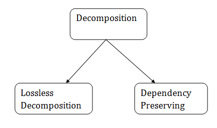
1. Lossless Decomposition

Lossless decomposition ensures that no information is lost when a relation is decomposed. It guarantees that the join of relations will result in the same relation as it was decomposed.

Key Points:

If no information is lost during the decomposition, it's considered lossless.
The join of decomposed relations should yield the original relation.
A relation is considered to have a lossless decomposition if the natural joins of all the decompositions give the original relation.

Example:

Consider the "EMPLOYEE_DEPARTMENT" table:

EMP_ID	EMP_NAME	EMP_AGE	EMP_CITY	DEPT_ID	DEPT_NAME
22	Denim	28	Mumbai	827	Sales
33	Alina	25	Delhi	438	Marketing
46	Stephan	30	Bangalore	869	Finance
52	Katherine	36	Mumbai	575	Production
60	Jack	40	Noida	678	Testing

This relation is decomposed into two relations: "EMPLOYEE" and "DEPARTMENT."

EMPLOYEE table:

EMP_ID	EMP_NAME	EMP_AGE	EMP_CITY
22	Denim	28	Mumbai
33	Alina	25	Delhi
46	Stephan	30	Bangalore
52	Katherine	36	Mumbai
60	Jack	40	Noida

DEPARTMENT table:

DEPT_ID	EMP_ID	DEPT_NAME
827	22	Sales
438	33	Marketing
869	46	Finance
575	52	Production
678	60	Testing

When these two relations are joined on the common column "EMP_ID," the resultant relation is the same as the original relation:

Employee ⋈ Department

EMP_ID	EMP_NAME	EMP_AGE	EMP_CITY	DEPT_ID	DEPT_NAME
22	Denim	28	Mumbai	827	Sales
33	Alina	25	Delhi	438	Marketing
46	Stephan	30	Bangalore	869	Finance
52	Katherine	36	Mumbai	575	Production
60	Jack	40	Noida	678	Testing

Hence, the decomposition is a lossless join decomposition.

2. Dependency Preserving

Dependency preserving is an essential constraint of a database design.

Key Points:

At least one decomposed table must satisfy every dependency.
If a relation R is decomposed into relations R1 and R2, the dependencies of R must either be a part of R1 or R2 or must be derivable from the combination of functional dependencies of R1 and R2.

For example, suppose there is a relation R (A, B, C, D) with a functional dependency set (A -> BC). The relational R is decomposed into R1 (ABC) and R2 (AD), which is dependency preserving because the FD A -> BC is a part of relation R1 (ABC).

Normalization

Database normalization is the process of organizing the attributes of the database to reduce or eliminate data redundancy (having the same data but at different places).

Problems because of data redundancy: Data redundancy unnecessarily increases the size of the database as the same data is repeated in many places. Inconsistency problems also arise during insert, delete and update operations.

Normalization is the process of organizing the data in the database.
Normalization is used to minimize the redundancy from a relation or set of relations. It is also used to eliminate undesirable characteristics like Insertion, Update, and Deletion Anomalies.
Normalization divides the larger table into smaller and links them using relationships.
The normal form is used to reduce redundancy from the database table.

The main reason for normalizing the relations is removing these anomalies. Failure to eliminate anomalies leads to data redundancy and can cause data integrity and other problems as the database grows. Normalization consists of a series of guidelines that helps to guide you in creating a good database structure.

Data modification anomalies can be categorized into three types:

Insertion Anomaly: Insertion Anomaly refers to when one cannot insert a new tuple into a relationship due to lack of data.
Deletion Anomaly: The delete anomaly refers to the situation where the deletion of data results in the unintended loss of some other important data.
Updatation Anomaly: The update anomaly is when an update of a single data value requires multiple rows of data to be updated.

Advantages of Normalization

Normalization helps to minimize data redundancy.
Greater overall database organization.
Data consistency within the database.
Much more flexible database design.
Enforces the concept of relational integrity.

Disadvantages of Normalization

You cannot start building the database before knowing what the user needs.
The performance degrades when normalizing the relations to higher normal forms, i.e., 4NF, 5NF.
It is very time-consuming and difficult to normalize relations of a higher degree.
Careless decomposition may lead to a bad database design, leading to serious problems.

1NF, 2NF, 3NF, BCNF, 4NF

Normal Form	Description
1NF	A relation is in 1NF if it contains an atomic value.
2NF	A relation will be in 2NF if it is in 1NF and all non-key attributes are fully functional dependent on the primary key.
3NF	A relation will be in 3NF if it is in 2NF and no transition dependency exists.
BCNF	A stronger definition of 3NF is known as Boyce Codd's normal form.
4NF	A relation will be in 4NF if it is in Boyce Codd's normal form and has no multi-valued dependency.
5NF	A relation is in 5NF if it is in 4NF and does not contain any join dependency; joining should be lossless.

1. First Normal Form (1NF)

If a relation contains a composite or multi-valued attribute, it violates the first normal form, or the relation is in first normal form if it does not contain any composite or multi-valued attribute. A relation is in first normal form if every attribute in that relation is singled valued attribute.

A table is in 1 NF if:

There are only Single Valued Attributes.
Attribute Domain does not change.
There is a unique name for every Attribute/Column.
The order in which data is stored does not matter.

Example:

Original Table (Not in 1NF):

ID	Name	Courses
1	A	c1, c2
2	E	c3
3	M	c2, c3

In the above table, the "Courses" column is a multi-valued attribute, so it is not in 1NF.

Table in 1NF (Each Course as a Separate Row):

ID	Name	Course
1	A	c1
1	A	c2
2	E	c3
3	M	c2
3	M	c3

Note: A database design is considered bad if it is not even in the First Normal Form (1NF).

2. Second Normal Form (2NF)

Second Normal Form (2NF): Second Normal Form (2NF) is based on the concept of full functional dependency. Second Normal Form applies to relations with composite keys, that is, relations with a primary key composed of two or more attributes. A relation with a single-attribute primary key is automatically in at least 2NF.

Example-:

Consider the following functional dependencies in relation R (A, B, C, D):

AB -> C [A and B together determine C]
BC -> D [B and C together determine D]

In this case, we can see that the relation R has a composite candidate key {A, B} as AB -> C. Therefore, A and B together uniquely determine the value of C. Similarly, BC -> D shows that B and C together uniquely determine the value of D.

The relation R is already in 1NF because it does not have any repeating groups or nested relations.

However, we can see that the non-prime attribute D is functionally dependent on only part of a candidate key, BC. This violates the 2NF condition.

3. Third Normal Form (3NF):

A relation will be in 3NF if it is in 2NF and does not contain any transitive partial dependency.
3NF is used to reduce data duplication and achieve data integrity.
If there is no transitive dependency for non-prime attributes, then the relation must be in the third normal form.

Conditions for 3NF: For every non-trivial functional dependency X → Y, a relation is in 3NF if it holds at least one of the following conditions: 1. X is a super key. 2. Y is a prime attribute, i.e., each element of Y is part of some candidate key.

Example:

Consider the "EMPLOYEE_DETAIL" table:

EMP_ID	EMP_NAME	EMP_ZIP	EMP_STATE	EMP_CITY
222	Harry	201010	UP	Noida
333	Stephan	02228	US	Boston
444	Lan	60007	US	Chicago
555	Katharine	06389	UK	Norwich
666	John	462007	MP	Bhopal

Super key in the table above: {EMP_ID}, {EMP_ID, EMP_NAME}, {EMP_ID, EMP_NAME, EMP_ZIP}, and so on.
Candidate key: {EMP_ID}
Non-prime attributes: In the given table, all attributes except EMP_ID are non-prime.
Here, EMP_STATE & EMP_CITY are dependent on EMP_ZIP, and EMP_ZIP is dependent on EMP_ID. The non-prime attributes (EMP_STATE, EMP_CITY) transitively depend on the super key (EMP_ID), violating the rule of the third normal form.

To achieve 3NF, we need to move EMP_CITY and EMP_STATE to a new "EMPLOYEE_ZIP" table, with EMP_ZIP as the Primary key.

EMPLOYEE table:

EMP_ID	EMP_NAME	EMP_ZIP
222	Harry	201010
333	Stephan	02228
444	Lan	60007
555	Katharine	06389
666	John	462007

EMPLOYEE_ZIP table:

EMP_ZIP	EMP_STATE	EMP_CITY
201010	UP	Noida
02228	US	Boston
60007	US	Chicago
06389	UK	Norwich
462007	MP	Bhopal

This separation of data into two tables (EMPLOYEE and EMPLOYEE_ZIP) satisfies the third normal form and eliminates transitive dependencies.

4.Boyce-Codd Normal Form (BCNF):

Boyce--Codd Normal Form (BCNF) is a level of normalization in database design that considers all candidate keys in a relation. BCNF has additional constraints compared to the general definition of 3NF.

Rules for BCNF:

Rule 1: The table should be in the 3rd Normal Form (3NF).
Rule 2: X should be a superkey for every functional dependency (FD) X → Y in a given relation.

How to Satisfy BCNF:

To satisfy BCNF, a table may need to be decomposed into further tables. Here is the full procedure for transforming a table into BCNF. Let's start by dividing the main table into two tables: "Stu_Branch" and "Stu_Course" tables.

Stu_Branch Table:

Stu_ID	Stu_Branch
101	Computer Science & Engineering
102	Electronics & Communication Engineering

Candidate Key for this table: Stu_ID.

Stu_Course Table:

Stu_Course	Branch_Number	Stu_Course_No
DBMS	B_001	201
Computer Networks	B_001	202
VLSI Technology	B_003	401
Mobile Communication	B_003	402

Candidate Key for this table: Stu_Course.

Stu_ID to Stu_Course_No Table:

Stu_ID	Stu_Course_No
101	201
101	202
102	401
102	402

Candidate Key for this table: {Stu_ID, Stu_Course_No}.

After decomposing the main table into further tables, it is now in BCNF as it satisfies the condition that X is a superkey for every functional dependency X → Y.

This decomposition ensures that the BCNF requirements are met and helps in achieving a well-structured and normalized database design.

Query Optimization:

Query optimization is of great importance for the performance of a relational database, especially for the execution of complex SQL statements. A query optimizer decides the best methods for implementing each query.

The query optimizer selects, for instance, whether or not to use indexes for a given query, and which join methods to use when joining multiple tables. These decisions have a tremendous effect on SQL performance, and query optimization is a key technology for every application, from operational systems to data warehouses and analytical systems to content management systems.

Principles of Query Optimization:

Understand the Query Execution: The first phase of query optimization is understanding what the database is performing. Different databases have different commands for this. For example, in MySQL, one can use the "EXPLAIN [SQL Query]" keyword to see the query plan. In Oracle, one can use the "EXPLAIN PLAN FOR [SQL Query]" to see the query plan.
Retrieve as Little Data as Possible: Minimize the amount of data retrieved from the database. The more information retrieved from the query, the more resources the database needs to process and store. Avoid using 'SELECT *' when only specific columns are needed.
Store Intermediate Results: For complex queries, consider using subqueries, inline views, and UNION-type statements to generate intermediate results. These transitional results are not saved in the database but are directly used within the query. Be cautious when dealing with large transitional results, as they can impact performance.

Query Optimization Strategies:

Use Index: Utilize indexing as the primary strategy to speed up a query. Well-designed indexes can significantly improve query performance.
Aggregate Tables: Pre-populate tables at higher levels to reduce the amount of data that needs to be processed during query execution.
Vertical Partitioning: Partition tables by columns to reduce the amount of data a SQL query needs to process.
Horizontal Partitioning: Partition tables by data value, often based on time, to reduce the data volume processed by SQL queries.
De-normalization: Combine multiple tables into a single table to reduce the need for extensive table joins, thereby speeding up query execution.
Server Tuning: Adjust server parameters to fully utilize hardware resources, improving query execution speed. Server tuning is specific to each server's hardware and software configuration.

Query optimization is a critical aspect of database performance tuning, and applying these principles and strategies can lead to significant improvements in SQL query performance.

Components of Query Optimizer:

The query optimizer consists of three components: 1. Query Transformer: Determines if it's advantageous to change original SQL statements into less expensive, semantically equivalent SQL statements. 2. Estimator: Calculates the overall cost of an execution plan, using techniques like selectivity (row selectivity based on query predicates), cardinality (number of rows returned by each action), and cost (measuring resource usage). 3. Plan Generator: Generates feasible execution plan designs due to multiple combinations available for achieving the same goal.

Automatic Tuning Optimizer:

The optimizer performs various operations depending on how it is invoked. It offers different categories of optimizations: - Normal Optimization: Generates an execution strategy for SQL statements. It operates within tight time constraints and aims to choose the best plan. - SQL Tuning Advisor Optimization: Activated by SQL Tuning Advisor, it performs additional research to enhance plans created in regular mode. It generates a set of activities to create a better plan.

Methods of Query Optimization in DBMS:

Cost-Based Optimization: In cost-based optimization, the optimizer selects the most efficient way to execute a SQL statement. It calculates cost estimates for potential plans and chooses the plan with the lowest estimated cost. This method is also known as the Cost-Based Optimizer.

Execution Plans: Describe the actions taken by the database to execute a SQL statement. Each operation in the plan has a cost associated with it.
Query Blocks: Internally, the optimizer uses query blocks to represent SELECT blocks in the original SQL statement. Query blocks are used to optimize parts of the query individually.

Adaptive Query Optimizer in DBMS:

Adaptive query optimization allows the optimizer to modify execution plans in real-time and learn new facts that can improve statistics. It's useful when available data is insufficient for generating a perfect plan.

Adaptive plans are significant because they help avoid subpar default plans due to incorrect cardinality estimation. The optimizer can adjust the plan as it's being executed based on actual execution statistics, resulting in a more ideal final plan. This final plan is then used for further executions, ensuring that subpar plans are not reused.

References

https://www.javatpoint.com/dbms-functional-dependency
https://www.tutorialspoint.com/dbms/database_normalization.htm
https://www.geeksforgeeks.org/functional-dependency-and-attribute-closure/?ref=lbp
https://minigranth.in/dbms-tutorial/closure-of-functional-dependency
https://www.javatpoint.com/dbms-normalization
https://www.geeksforgeeks.org/introduction-of-database-normalization/?ref=lbp
https://www.geeksforgeeks.org/first-normal-form-1nf/?ref=lbp
https://www.geeksforgeeks.org/second-normal-form-2nf/?ref=lbp
https://www.javatpoint.com/dbms-third-normal-form
https://www.geeksforgeeks.org/boyce-codd-normal-form-bcnf/?ref=lbp
https://www.javatpoint.com/dbms-forth-normal-form
https://www.tutorialspoint.com/what-is-query-optimization
https://www.scaler.com/topics/query-optimization-in-dbms/
https://www.tutorialandexample.com/query-optimization-in-dbms